As mentioned in section 4.3.1,
ScaLAPACK assumes a one-dimensional or
two-dimensional block-cyclic distribution
for the dense matrix computational routines.
The block-cyclic distribution is
a generalization of the block and cyclic
distributions. In one dimension, blocks
of rows of size MB or blocks of columns
of size NB are cyclically distributed
over the processes. In two dimensions,
blocks of size ![]() are
distributed cyclically over the processes.
Example programs can be found in
section 2.3 and
Appendix C.1.
are
distributed cyclically over the processes.
Example programs can be found in
section 2.3 and
Appendix C.1.
According to the two-dimensional block
cyclic data distribution, scheme an M_
by N_
dense matrix is first decomposed into MB_
by NB_
blocks starting at its upper left corner.
These blocks are then uniformly distributed
in each dimension of the process grid. Thus,
every process owns a collection of blocks,
which are locally and contiguously stored
in a two-dimensional ``column major'' array.
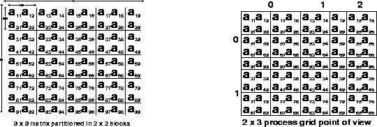
The partitioning of a ![]() matrix into
matrix into
![]() blocks and the mapping
of these blocks onto a
blocks and the mapping
of these blocks onto a ![]() process grid are shown in figure 4.6.
The local entries of every matrix
column are contiguously stored in
the processes' memories.
process grid are shown in figure 4.6.
The local entries of every matrix
column are contiguously stored in
the processes' memories.

Figure: 4.6 A ![]() matrix decomposed into
matrix decomposed into ![]() blocks mapped onto a
blocks mapped onto a ![]() process grid
process grid
The number of rows of a matrix
and the number of columns of a
matrix that a specific process
owns, denoted LOC![]() and
LOC
and
LOC![]() respectively, may
differ from process to process
in the process grid. Likewise,
there is a local leading
dimension LLD_
for each process in the process
grid. This value may be different
on each process in the process
grid. For example, we can see
on the right of figure 4.6
that the local array stored in
process row 0 must have a local
leading dimension LLD_
greater than or equal to 5, and
greater than or equal to 4 in the
process row 1.
respectively, may
differ from process to process
in the process grid. Likewise,
there is a local leading
dimension LLD_
for each process in the process
grid. This value may be different
on each process in the process
grid. For example, we can see
on the right of figure 4.6
that the local array stored in
process row 0 must have a local
leading dimension LLD_
greater than or equal to 5, and
greater than or equal to 4 in the
process row 1.

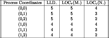
Table 4.8: Sizes of the local arrays
Table 4.8 gives the values of the local array sizes associated with figure 4.6.