HPL Algorithm

This page provides a high-level description of the algorithm used in this package. As indicated below, HPL contains in fact many possible variants for various operations. Defaults could have been chosen, or even variants could be selected during the execution. Due to the performance requirements, it was decided to leave the user with the opportunity of choosing, so that an "optimal" set of parameters could easily be experimentally determined for a given machine configuration. From a numerical accuracy point of view, all possible combinations are rigorously equivalent to each other even though the result may slightly differ (bit-wise).

Main Algorithm

This software package solves a linear system of order n: A x = b by first computing the LU factorization with row partial pivoting of the n-by-n+1 coefficient matrix [A b] = [[L,U] y]. Since the lower triangular factor L is applied to b as the factorization progresses, the solution x is obtained by solving the upper triangular system U x = y. The lower triangular matrix L is left unpivoted and the array of pivots is not returned.

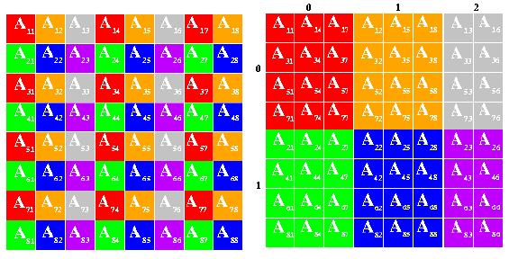
The data is distributed onto a two-dimensional P-by-Q grid of processes according to the block-cyclic scheme to ensure "good" load balance as well as the scalability of the algorithm. The n-by-n+1 coefficient matrix is first logically partitioned into nb-by-nb blocks, that are cyclically "dealt" onto the P-by-Q process grid. This is done in both dimensions of the matrix.

The right-looking variant has been chosen for the main loop of the LU factorization. This means that at each iteration of the loop a panel of nb columns is factorized, and the trailing submatrix is updated. Note that this computation is thus logically partitioned with the same block size nb that was used for the data distribution.

Panel Factorization

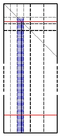
At a given iteration of the main loop, and because of the cartesian property of the distribution scheme, each panel factorization occurs in one column of processes. This particular part of the computation lies on the critical path of the overall algorithm. The user is offered the choice of three (Crout, left- and right-looking) matrix-multiply based recursive variants. The software also allows the user to choose in how many sub-panels the current panel should be divided into during the recursion. Furthermore, one can also select at run-time the recursion stopping criterium in terms of the number of columns left to factorize. When this threshold is reached, the sub-panel will then be factorized using one of the three Crout, left- or right-looking matrix-vector based variant. Finally, for each panel column the pivot search, the associated swap and broadcast operation of the pivot row are combined into one single communication step. A binary-exchange (leave-on-all) reduction performs these three operations at once.

Panel Broadcast

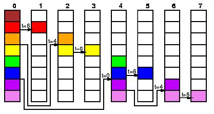
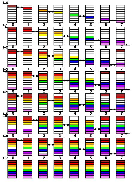
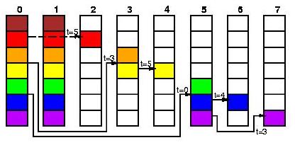
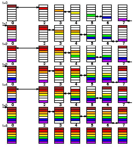
Once the panel factorization has been computed, this panel of columns is broadcast to the other process columns. There are many possible broadcast algorithms and the software currently offers 6 variants to choose from. These variants are described below assuming that process 0 is the source of the broadcast for convenience. "->" means "sends to".

Increasing-ring: 0 -> 1; 1 -> 2; 2 -> 3 and so on. This algorithm is the classic one; it has the caveat that process 1 has to send a message.
Increasing-ring (modified): 0 -> 1; 0 -> 2; 2 -> 3 and so on. Process 0 sends two messages and process 1 only receives one message. This algorithm is almost always better, if not the best.
Increasing-2-ring: The Q processes are divided into two parts: 0 -> 1 and 0 -> Q/2; Then processes 1 and Q/2 act as sources of two rings: 1 -> 2, Q/2 -> Q/2+1; 2 -> 3, Q/2+1 -> to Q/2+2 and so on. This algorithm has the advantage of reducing the time by which the last process will receive the panel at the cost of process 0 sending 2 messages.
Increasing-2-ring (modified): As one may expect, first 0 -> 1, then the Q-1 processes left are divided into two equal parts: 0 -> 2 and 0 -> Q/2; Processes 2 and Q/2 act then as sources of two rings: 2 -> 3, Q/2 -> Q/2+1; 3 -> 4, Q/2+1 -> to Q/2+2 and so on. This algorithm is probably the most serious competitor to the increasing ring modified variant.
Long (bandwidth reducing): as opposed to the previous variants, this algorithm and its follower synchronize all processes involved in the operation. The message is chopped into Q equal pieces that are scattered across the Q processes. The pieces are then rolled in Q-1 steps. The scatter phase uses a binary tree and the rolling phase exclusively uses mutual message exchanges. In odd steps 0 <-> 1, 2 <-> 3, 4 <-> 5 and so on; in even steps Q-1 <-> 0, 1 <-> 2, 3 <-> 4, 5 <-> 6 and so on. More messages are exchanged, however the total volume of communication is independent of Q, making this algorithm particularly suitable for large messages. This algorithm becomes competitive when the nodes are "very fast" and the network (comparatively) "very slow".
Long (bandwidth reducing modified): same as above, except that 0 -> 1 first, and then the Long variant is used on processes 0,2,3,4 .. Q-1.

The rings variants are distinguished by a probe mechanism that activates them. In other words, a process involved in the broadcast and different from the source asynchronously probes for the message to receive. When the message is available the broadcast proceeds, and otherwise the function returns. This allows to interleave the broadcast operation with the update phase. This contributes to reduce the idle time spent by those processes waiting for the factorized panel. This mechanism is necessary to accomodate for various computation/communication performance ratio.

Look-ahead

Once the panel has been broadcast or say during this broadcast operation, the trailing submatrix is updated using the last panel in the look-ahead pipe: as mentioned before, the panel factorization lies on the critical path, which means that when the kth panel has been factorized and then broadcast, the next most urgent task to complete is the factorization and broadcast of the k+1 th panel. This technique is often refered to as "look-ahead" or "send-ahead" in the literature. This package allows to select various "depth" of look-ahead. By convention, a depth of zero corresponds to no lookahead, in which case the trailing submatrix is updated by the panel currently broadcast. Look-ahead consumes some extra memory to essentially keep all the panels of columns currently in the look-ahead pipe. A look-ahead of depth 1 (maybe 2) is likely to achieve the best performance gain.

Update

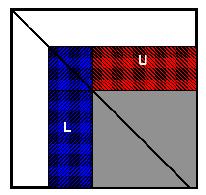
The update of the trailing submatrix by the last panel in the look-ahead pipe is made of two phases. First, the pivots must be applied to form the current row panel U. U should then be solved by the upper triangle of the column panel. U finally needs to be broadcast to each process row so that the local rank-nb update can take place. We choose to combine the swapping and broadcast of U at the cost of replicating the solve. Two algorithms are available for this communication operation.

Binary-exchange: this is a modified variant of the binary-exchange (leave on all) reduction operation. Every process column performs the same operation. The algorithm essentially works as follows. It pretends reducing the row panel U, but at the beginning the only valid copy is owned by the current process row. The other process rows will contribute rows of A they own that should be copied in U and replace them with rows that were originally in the current process row. The complete operation is performed in log(P) steps. For the sake of simplicity, let assume that P is a power of two. At step k, process row p exchanges a message with process row p+2^k. There are essentially two cases. First, one of those two process rows has received U in a previous step. The exchange occurs. One process swaps its local rows of A into U. Both processes copy in U remote rows of A. Second, none of those process rows has received U, the exchange occurs, and both processes simply add those remote rows to the list they have accumulated so far. At each step, a message of the size of U is exchanged by at least one pair of process rows.
Long: this is a bandwidth reducing variant accomplishing the same task. The row panel is first spread (using a tree) among the process rows with respect to the pivot array. This is a scatter (V variant for MPI users). Locally, every process row then swaps these rows with the the rows of A it owns and that belong to U. These buffers are then rolled (P-1 steps) to finish the broadcast of U. Every process row permutes U and proceed with the computational part of the update. A couple of notes: process rows are logarithmically sorted before spreading, so that processes receiving the largest number of rows are first in the tree. This makes the communication volume optimal for this phase. Finally, before rolling and after the local swap, an equilibration phase occurs during which the local pieces of U are uniformly spread across the process rows. A tree-based algorithm is used. This operation is necessary to keep the rolling phase optimal even when the pivot rows are not equally distributed in process rows. This algorithm has a complexity in terms of communication volume that solely depends on the size of U. In particular, the number of process rows only impacts the number of messages exchanged. It will thus outperforms the previous variant for large problems on large machine configurations.

The user can select any of the two variants above. In addition, a mix is possible as well. The "binary-exchange" algorithm will be used when U contains at most a certain number of columns. Choosing at least the block size nb as the threshold value is clearly recommended when look-ahead is on.

Backward Substitution

The factorization has just now ended, the back-substitution remains to be done. For this, we choose a look-ahead of depth one variant. The right-hand-side is forwarded in process rows in a decreasing-ring fashion, so that we solve Q * nb entries at a time. At each step, this shrinking piece of the right-hand-side is updated. The process just above the one owning the current diagonal block of the matrix A updates first its last nb piece of x, forwards it to the previous process column, then broadcast it in the process column in a decreasing-ring fashion as well. The solution is then updated and sent to the previous process column. The solution of the linear system is left replicated in every process row.

Checking the Solution

To verify the result obtained, the input matrix and right-hand side are regenerated. The normwise backward error (see formula below) is then computed. A solution is considered as "numerically correct" when this quantity is less than a threshold value of the order of 1.0. In the expression below, eps is the relative (distributed-memory) machine precision.

|| Ax - b ||_oo / ( eps * ( || A ||_oo * || x ||_oo + || b ||_oo ) * n )

[Home] [Copyright and Licensing Terms] [Algorithm] [Scalability] [Performance Results] [Documentation] [Software] [FAQs] [Tuning] [Errata-Bugs] [References] [Related Links]